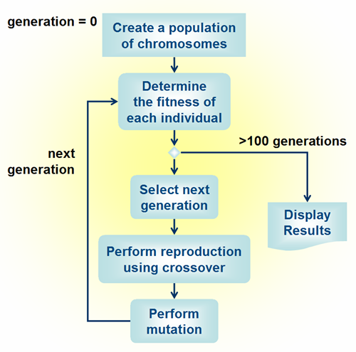
The basic algorithm by which GAs operate is reasonably well established. The
above figure shows the generic one used by most, although some variations may
occur depending on the application. In general the particular methods employed
in each of the above stages do not matter. What is important is that the general
algorithm is followed and the evolutionary techniques that underlie it are
understood. The following sections discuss the need for each of these steps in
terms of their relevance to evolutionary processes.
Population
A population is initiated of legal solutions, selected by choosing random
input values. There are no fixed rules for how large the population should be.
The answer is dependent upon the type of problem. For a simple problem with a
regular search space a small population of 40 to 100 will probably be
sufficient. For larger more complex problems and especially those with an
irregular search space larger populations of 400 or more are recommended. The
clue is diversity – a diverse population, i.e. a large one will tend to search
out niches – in engineering terms that means finding elusive, difficult to find
solutions to problems.
Fitness
The fitness of individual chromosomes is a relative matter. For example when
maximising a function; if one individual has a higher value, once processed by
the function, than another then that individual is considered fitter. Things get
a little more involved with multi-criteria problems. In these cases comparisons
can be carried out to see if an individual dominates other members of a
population by taking all criteria into consideration. If they do they are
considered fitter. The most dominant, i.e. those who dominate all others, are
referred to as Pareto solutions. These are considered as candidate solutions to
whatever problem you are trying to solve.
Selection of the Fittest
GAs operate over a number of generations. Following the evolutionary theme of
this method, this means fitter solutions will tend to survive to the next
generation. The selection method employed by many approaches is the roulette wheel
selection process. In
nature all individuals have a chance of surviving from one generation to the
next – fitter solutions (i.e. those most dominant) have a better chance. Weaker
more dominated individuals have a smaller chance (still an opportunity) of
surviving.
Nature generates the next generation using a mating process. As a result two
parents create offspring, who consist of the genetic material of both parents.
These offspring can be weaker or fitter than their parents (or similar). If they
are weaker they will tend to die out – if they are stronger their chances of
survival are better. GAs try to replicate this using a crossover operator. This emulates the
mating process by exchanging chromosome patterns between individuals to create
offspring for the next generation.
Mutation exists in nature and causes an unanticipated change in a
chromosome pattern. This can result in a much weakened individual and
occasionally a much stronger one. Either way the principle behind mutation from
an evolutionary point of view is that it occurs rarely, spontaneously and
without reference to any other individual in the population. If the change is
beneficial to the general population then that individual will tend to survive
and will pass this trait on in future replication processes. Because of the way
that GAs represent individuals this process is a very simple one and a typical
mutation operator is relatively easy
to implement. It is important to remember that these processes occur very
infrequently otherwise they would have a disruptive effect on the overall
population.
There are no definitive methods of establishing how many generations a GA
should run for. Simple problems may converge on good solutions after only 20 or
30 generations. More complex problems may need more. It is not unusual to run a
GA for 400 generations for more complex problems such as jobshops. The above
figure suggests 100 generations. The most reliable method of deciding on this is
trial and error, although a number of authors have suggested methods for
determining how long a solution should live.
For further details of the EDC's activities please get in touch
with us through our contact page.
void CMessageMapDlg::DoDataExchange(CDataExchange* pDX)
{
CDialog::DoDataExchange(pDX);
//{{AFX_DATA_MAP(CMessageMapDlg)
// NOTE: the ClassWizard will add DDX and DDV calls here
//}}AFX_DATA_MAP
}
이 부분은 버튼의 ID와 핸들러 함수를 연결시키는 매크로입니다. ON_BN_CLICKED 부분이 매크로구요,
IDC_BUTTON1 부분은 버튼의 ID , OnButton1은 그 버튼에 대한 핸들러 함수이죠. 버튼을 5개 놓았으므로
연결시키는 매크로 부분이 5개가 됩니다.
7. 만약 버튼이 100개라면 위와 같은 매크로가 100개가 만들어져야
하고, 그에 따라 핸들러 함수도 100개가 만들어지겠죠. 상당한 노가다가 아닐 수 없습니다. 이걸 좀더 단순하게 줄이기 위해서
다른 매크로를 사용하면 됩니다. ON_CONTROL_EX 나 ON_CONTROL_RANGE 같은 매크로 말이죠.
이것에 대해 알아보기 전에 다음내용부터 먼저 알아보기로 하죠. 다음 방법을 사용해서 여러개의 핸들러 함수를 하나로 줄일 수 있습니다.
---- X ---- X ---- X ----
7.1 ON_BN_CLICKED 매크로는 afxmsg_.h 파일을 보면 다음처럼 정의되어 있습니다.

 uosu160.rar


 HotSwap! 4.5.0.0.ZIP